
Research Article
Estimating Probabilities, Odds and Odds Ratios in Gestational Outcomes: A Dummy Variable Regression Illustration
1 Department of Industrial Mathematics and Health Statistics, David Umahi Federal University of Health Sciences, Ebonyi State, Nigeria.
2 International Institute for Nuclear Medicine and Allied Health Research, David Umahi Federal University of Health Sciences, Ebonyi State, Nigeria.
*Corresponding Author: Uchechukwu Marius Okeh, Department of Industrial Mathematics and Health Statistics, David Umahi Federal University of Health Sciences, Ebonyi State, Nigeria.
Citation: Okeh UM, Igwe TS, Okpara PA. (2025). Estimating Probabilities, Odds and Odds Ratios in Gestational Outcomes: A Dummy Variable Regression Illustration, Journal of BioMed Research and Reports, BioRes Scientia Publishers. 8(6):1-16. DOI: 10.59657/2837-4681.brs.25.210
Copyright: © 2025 Mathias Adawurah, this is an open-access article distributed under the terms of the Creative Commons Attribution License, which permits unrestricted use, distribution, and reproduction in any medium, provided the original author and source are credited.
Received: September 23, 2025 | Accepted: October 06, 2025 | Published: October 13, 2025
Abstract
Dummy variable regression model assumes a linear relationship between the categorical predictor variables (e.g., maternal age, parity and infant gender) and outcome variable here called gestation length. Similarly, the coefficients resulting from dummy variable regression might not be directly interpretable in terms of probability changes or odds ratios, which may potentially limit the usefulness of the model. This might not hold true if the gestation length is binary/dichotomous. This study explores an alternative method of estimating probabilities, odds and odds ratios in gestational outcomes rather than the use of logistic regression. Dummy variable regression as the alternative approach can achieve these fit when the outcome predictor variable is continuous. The method involves first partitioning each of the parent independent variables into a set of mutually exclusive categories or subgroups and then use dummy variables to represent these categories in a regression model. In such a regression model, each parent independent variable is represented by one dummy variable of 1’s and 0’s less than the number of its categories. Any level of a parent independent variable that is not specifically represented by a dummy variable is referred to as the excluded level of that parent variable while the others are termed the included levels in the regression model. As part of the limitation of this study, there is need to ensure that the model assumptions are met, including linearity and independence of observations, continuity of the outcome variable as well as categorical nature of the predictor variables. To illustrate this method, a pilot cross sectional study design was carried out at Alex Ekwueme Federal University Teaching Hospital Abakaliki where data was collected from 41 anti-natal women with information regarding their age, parity and sex of last births harvested from them. Data analysis was done using SPSS version 14. The overall results of analysis showed that which indicated an insignificant relationship between the outcome variable and the categorical predictor variables, signaling the end of analysis but for illustration purposes only, probabilities can be estimated and after words, any desired odds and odds ratios like the odds that the randomly selected mother has a male and female births with gestation period of more than 39.5 weeks gave 0.636 and 0.639 as odds for male and female respectively while odds ratio was 0.995 implying that for every 1000 female births with a gestation length of more than 39.5 weeks, there are 995 males’ births with the same gestation period of 39.5 weeks. Also note for example that implies that if maternal age and gender of child are held at constant levels (made zeros), then the probability is 14.5 percent higher on the average for a randomly selected mother with a parity of two or three children when compared with other mothers that the gestation length of her last birth exceeds 39.5 weeks. We conclude that dummy variable regression enables one to estimate probabilities, odds and odds ratios of continuous outcome variable. As an alternative method to logistic regression, it compares favorably. Based on this approach, any desired probabilities, odds and odds ratios can be estimated.
Keywords: odds; odds ratio; continuous outcome; dummy variable regression; probabilities; maternal age
Introduction
Several researchers use the concept of multiple regression analysis and ANOVA in their statistical research analysis. Multiple regression analysis is frequently used in different aspects of life. Analyzed University model using multiple regression and ANCOVA and found the model very essential [1]. A researcher studied the significance of active-employment programs on employment levels using multiple regression [2]. It was also shown how viewing multiple regression results through multiple lenses can give a better assessment to the researchers [3]. Again, using multiple regression to obtain accurate parameter contributes more than having statistical significance [4]. Suppressor variables and suppression effects in building regression model was studied [5]. All of these were how multiple regression can be utilized in research to achieve some goals.
Often subject or candidate for an examination or job interview may wish to estimate the probability of success given some predisposing factors such as the number of hours the subject studied per day or per week, the nature, type and duration of the examination, the candidates’ prior qualifications, age, gender, ethnic group, state of origin, etc. A Clinician conducting a diagnostic test or drug trial for a certain condition may wish to know the odds that subjects or patients respond positive given their various characteristics such as age, gender, body weight, family history, etc. A Gynecologist or Pediatrician may wish to estimate the odds that a new born baby is under-weight or has more than normal gestation period even given the mothers’ age, parity, body weight and the Childs’ gender. etc. In other words, the response (outcome variable) to the condition of interest may be continuous having values/numbers that are both in whole and decimal places or binary/dichotomous assuming one of two possible values and the predisposing factors are either categorical variables or could be subdivided into a number of mutually exclusive sub-groups or classes. This would hence enable the fitting of a multiple regression model in which the dependent (outcome variable) and independent (explanatory) variables are continuous and categorical respectively. These will enable one to estimate the probabilities, odds and odds ratios of occurrence of the outcome of interest using dummy variable regression as hereunder discussed.
Statement of Problem
Overtime the use of logistic regression in estimating probabilities and odds ratios of occurrence of the outcome of interest has dominated almost every research work which made one to wonder if it is not possible to find an alternative approach to it. It is therefore necessary to know some of the problem statement involved in research like this and how there can be tackled: (a). Dummy variable regression model is not the best fit for analyzing the gestation length data if the outcome variable is binary (e.g., preterm birth yes/no) or categorical (e.g., preterm/term/post term). Available literature reveals the use of logistic regression or multinomial logistic regression models for their analysis. For dummy variable regression model to be applicable, the outcome variable must be continuous while the predictor variables should be categorical in nature. This is entirely a new area of research for use in gestation length data. (b). Dummy variable regression model assumes a linear relationship between the categorical predictor variables (maternal age, parity and infant gender) and outcome variable here called gestation length. This might not hold true if the gestation lengths are binary/dichotomous. Since the outcome variable is continuous, the relationship becomes linear when dummy variable regression is applied. (c). Coefficients resulting from dummy variable regression might not be directly interpretable in terms of probability changes or odds ratios, which may potentially limit the usefulness of the model. These issues are resolved simply given the continuous nature of the outcome variable (gestation length in range of values) as well as the categorical nature of the predictor variables (parity-primipara/multipara, maternal age;23 years or less/26-29 years and infant gender; male/female). These nature enables a clear and simple interpretation of the interaction effects of the continuous outcome variable and the categorical variables devoid of confusion. (d). The fact that the use of logistic regression dominated available literature in accurately predicting probabilities or odds ratios does not mean that dummy variable regression cannot achieve a good result when applied. The conditions and distinctions in the use of both models are clear and free from complexity.
Why Dummy Variable Regression is Preferable to Logistic Regression in This Study
We proposed dummy variable regression for this study based on the following points: (a) Dummy variable model is suitable for use in this study because the outcome variable (gestation length) is continuous and the predictor variables are categorical (e.g., parity: primipara/multipara, Gender: male/female, maternal Age:25 years or less/ from 26-29 years) in nature. Logistic regression is suitable for binary outcome variable. (b) The outcome variable is continuous because it is measured in weeks and days, providing a continuous scale. Note also that ultrasound estimates of gestation length can provide precise measurements, further supporting the continuous nature of gestation length. It is continuous since the range of values of gestation length is from approximately 20 weeks to 42 weeks with many possible values in between. It is also in decimal values, e.g,39.5 weeks allowing for precise estimates. (c) Dummy variable regression allows for interaction effects between categorical predictor variables and continuous outcome variable. (d) Dummy variable regression considers linear relationship between outcome variable/dependent and independent (predictor) variables.
Limitations of Study
Some of the limitations of this study are: (a) The accuracy of the study relied heavily on the quality of the data collected. Poor data quality may lead to biased or incorrect estimates. (b) The distribution of the data may not meet the assumptions of the dummy variable regression model, potentially affecting the validity of the results. (c) Interpreting odds ratios can be complex, especially when dealing with multiple categories or interaction effects. (d) The study's results may be influenced by contextual factors not captured in the model, such as socioeconomic or environmental factors (e) The study's results may be specific to Ebonyi State and may not generalize to other regions of Nigeria or populations. (f) The study's results may be time-sensitive and may not remain valid over time due to changes in population demographics or healthcare practices. (g) The tendency to include too many dummy variables can naturally lead to multicollinearity. In this study, time were taken to address that issue by dropping some of the dummy variables.
Literature Review
Research works reviewed here are mainly those that utilized logistic regression in one way or the other in estimating probabilities and odds ratios since the use of dummy variable regression has not been made popular.
Logistic regression model of the dichotomous dependent variable and some covariates variables were used in estimating probabilities, odds and odds ratios of positive responses by engaging in a retrospective study on the effect of four independent risk factors (predictor variables) in the development of gestational diabetes mellitus (GDM) as outcome variable. The Odds ratio values for the risk factors showed significant relationship with the occurrence of GDM [6].
Odds ratio values were used to interpret the influence of the independent variables (educated and trained labor, uneducated and unskilled labor) on the dependent variable (the university choice). The results indicated that the chosen logistic regression model provided a significant improvement over a baseline model [7].
Hua and colleagues [8] provided a comprehensive and clinically relevant synthesis of logistic regression applications in clinical medicine, particularly in risk prediction and diagnostic modeling by evaluating best practices, addressing common pitfalls, and outlining validation techniques when using logistic regression to analyze binary outcomes such as disease presence versus absence. The review synthesized data from 41 peer-reviewed articles spanning from 1987 to 2025, selected from databases including PubMed, MEDLINE, and Scopus using some keywords. Results revealed that logistic regression remains a cornerstone technique in clinical risk prediction due to its interpretability and robust framework for handling binary outcomes. Findings indicate that logistic regression models, when appropriately validated, significantly enhance diagnostic accuracy and provide reliable risk estimates through odds ratios and confidence intervals. They concluded that logistic regression is an indispensable tool in clinical research for predicting binary outcomes and informing evidence-based practice.
Two researchers reviewed three common methods of estimating predicted probabilities following confounder-adjusted logistic regression. These methods are marginal standardization; prediction at the modes; and prediction at the means. Using an applied example, they demonstrated discrepancies in predicted probabilities across these methods. Results concluded that marginal standardization is the appropriate method when making inference to the overall population [9].
It was designed to model the factors impacting the actual milk yield of Holstein–Friesian cows using the proportional odds ordered logit model (OLM). The actual milk yield, the outcome variable, was categorized into three levels: low (< 4500> 7500 kg). The studied predictor variables were age at first calving (AFC), lactation order (LO), days open (DO), lactation period (LP), peak milk yield (PMY), and dry period (DP). The proportionality assumption of odds using the logit link function was verified for the current datasets. The goodness-of-fit measures revealed the suitability of the ordered logit models to datasets structure. The peak yield per kg was significantly related to the actual yield (P < 0>
Some scholars dichotomized count data into binary form and applied the logistic regression technique to estimate the OR. In other to ensure that there is no loss of information about the underlying counts which can reduce the precision of inferences on the OR, they proposed analyzing the count data directly using regression models with the log odds link function. With this approach, the parameter estimates in the model had the exact same interpretation as in a logistic regression of the dichotomized data, yielding comparable estimates of the OR. They proved analytically, using the Fisher information matrix, that their approach produced more precise estimates of the OR than logistic regression of the dichotomized data. Using simulation studies and real-world datasets, it was concluded that more precise estimates of the OR can be obtained directly from the count data by using the log odds link function [11].
Zhou et al [12] explored risk factors for birth defects (including a broad range of specific defects). Their data were derived from the Population-based Birth Defects Surveillance System in Hunan Province, China, 2014-2020. The surveillance population included all live births, stillbirths, infant deaths, and legal termination of pregnancy between 28 weeks’ gestation and 42 days postpartum. The prevalence of birth defects (number of birth defects per 1000 infants) and its 95% confidence interval (CI) were calculated. Multivariate logistic regression analysis (method: Forward, Wald, α = 0.05) and adjusted odds ratios (ORs) were used to identify risk factors for birth defects. The presence or absence of birth defects (or specific defects) were used as the dependent variable, and eight variables (sex, residence, number of births, paternal age, maternal age, number of pregnancies, parity, and maternal household registration) were entered as independent variables. Results showed that seven variables (except for parity) were associated with birth defects (or specific defects). They concluded that several risk factors were associated with birth defects (including a broad range of specific defects). It was also seen that one risk factor may be associated with several defects, and one defect may be associated with several risk factors.
Two Nigerians modelled a categorical response i.e., pregnancy outcome in terms of some predictors. Using ordinal logistic regression model and three major factors viz., environmental (previous cesareans, service availability), behavioral (antenatal care, diseases) and demographic (maternal age, marital status and weight) that affected the outcomes of pregnancies (livebirth, stillbirth and abortion). Using the model, the data collected was analyzed and result showed good fit. The research concluded that the odds of being in either of these categories i.e., livebirth or stillbirth showed that women with baby’s weight less than 2.5 kg are 18.4 times more likely to have had a livebirth than are women with history of babies 2.5 kg. Age (older age and middle aged) women are one halve (1.5) more likely to occur than lower aged women, likewise, is antenatal, (high parity and low parity) are more likely to occur 1.5 times than nullipara [13].
Hossain [14] demonstrated the estimation of logistic regression model in finding the factors associated with the likelihood of skilled workers in the garment sector of Bangladesh. It was found that the variables, years of education, years of experience, wage rate, grade, and working years at the present company have significant positive effects on the logit of the outcome variable Y, but the variable age of the companies has a significant negative effect.
Usman et al [15] investigated the performance of two re-sampling methods (Bootstrap and Jackknife) relationship and significance of social-economic factors (age, gender, marital status and settlement) and modes of HIV/AIDS transmission to the HIV/AIDS spread. They used logistic regression model, to relate social-economic factors (age, sex, marital status and settlement) to HIV/AIDS spread. This statistical predictive model was used to project the likelihood response of HIV/AIDS spread with a larger population using 10,000 Bootstrap re-sampled observations and Jackknife re-sampled. Result showed that given the two re-sampling methods, one can conclude that HIV transmission in Kebbi state is higher among the married couples than single individuals and concentrate more in the rural areas.
Knowledge Gaps
The following gaps exists for this study: (a). There is limited knowledge and understanding of the assumptions underlying dummy variable regression model and how to apply it in estimating probabilities and odds ratios of length of gestation. (b). The identified difficulty in interpreting coefficients and odds ratios in the context of length of gestation especially for non-statisticians. (c). There is limited knowledge and understanding of how dummy variable regression model compares to other statistical models such as logistic regression and multinomial logistic regression models in analyzing data relating to length of gestation. (d). There is inadequate understanding of the requirements for data quality and preparation before using dummy variable regression. For instance, outcome variable has to be continuous while the predictor variables should be categorical for it to qualified for dummy variable regression analysis. (e). Inadequate consideration of contextual factors specific to Ebonyi State may influence length of gestation. Such factors can be socioeconomic or environmental.
Method
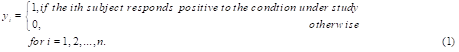
Suppose a researcher collects a random sample of size n respondent, subjects, or patients from a certain population; for investigation for the presence or absence of some condition. Let yi be the response of the ith subject to the condition under study in the presence of some predisposing factors on parent explanatory variables A, B, C,….with levels a,b,c…respectively for i=1,2,…,n.
Let
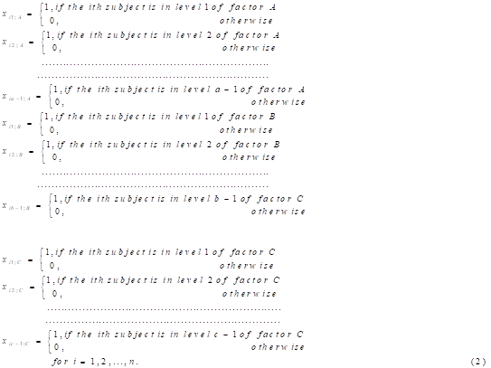
Interest is in representing each of the parent explanatory variables A, B, C, …. as dummy variables of 1s and 0s and using them in a multiple dummy variable regression model in which y is the dependent variable with two mutually exclusive outcomes. To do this each of the parent independent or explanatory variables is represented by one dummy variable less than the number of its categories or levels. This is to avoid linear dependence among the columns of the design matrix X of the regression model and hence ensure that X is of full column rank [16-18].
This let,
Following these specifications, we may now fit the multiple dummy variable regression model expressing the dependence of  on the
  as
as
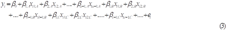
Where  are regression parameters or coefficients and
  are error terms uncorrelated with the
  with
with  for i=1,2,…,n. Note that Equation 3 may alternatively be represented in its matrix form as
Where 
is an nx1 column vector of 1’s and 0’s representing the n scores or responses of subjects to the condition of interest, X is an nxr design matrix of 1’s and 0’s,  is an rx1 column vector of regression parameters and
  is an nx1 column vector of error terms uncorrelated with X with
  where n is the number of parameters(regression coefficients) in the model (Equation 3).
Applying the method of least squares to either Equation 3 or 4 yields an unbiased estimator of as

The following analysis of variance (ANOVA) Table is used to test the adequacy of Equation 3 or 4 based on the F-test statistic.
Table 1: ANOVA Table for Equation 4.
| Source of Variation | Sum of Square (SS) | Degree of Freedom (DF) | Mean Sum of Square (MS) | F-Ratio |
| Regression |  | r-1 |  |  |
| Error |  | n-r |  | |
| Total |  | n-1 |
The null hypothesis to be tested for the adequacy of Equation 4 using the results of Table 1 is

 is rejected at the
  level of significance if

Otherwise is accepted where  is the critical value of F distribution with r-1 and n-r degrees of freedom for a specified of significance. If the model fits, that is if is rejected so that not all the are zero, then we may proceed to estimate the required probabilities and odds of positive responses to the condition of interest.
Now from Equation 4 we have that the expected value of y is

Or equivalently from Equation 3 we have that
Which is the expected proportion of positive responses or the probability that the ith subject responds positive (1) to the condition of interest. The expected probability that the ith subject responds negative (0) is

Hence the odds that the ith randomly selected subject responds positive to the condition under study is

In particular interest may be on some specific levels of some parent explanatory variable such as the jth level of factor A say. Then to find the probability that the ith randomly selected subject in the jth level of factor A responds positive to the condition we set  and all other
  in Equation 9 yielding
For j=1, 2,….,a-1
This is the probability that the jth level of factor A together with the omitted levels of all the other factors in the model (the levels) omitted in the specifications Equation 2 respond positive to the condition under study. Similarly, the probability that this subject (ith the jth level of factor A and omitted levels of the other factors) responds

Hence the odds that the ith randomly selected subject in the jth level of factor A and the omitted levels of the other factors responding positive to the condition under study is

Now that Equations 12 13 and 14 are obtained from Equations 9,10 and 11 respectively by certain

Equations 12 and 13 are respectively the probability that a randomly selected subject responds positives and the probability that the subject responds negative to the condition under study while Equation 14 is the odds of positive response. In general, if interest is in determining the odds of positive response by a randomly selected subject in the jth level of factor A, lth level of factor B, sth level of factor C and omitted levels of other factors in the model, 
Finally, the odds ratio of positive response or of experiencing the condition by a randomly selected subjects in the jth and kth levels of factor A and omitted levels of other factors in the model is
Results
Sample Size Justification
Why a sample size of 41 is justifiably used in this study are as follows:
(a). This is pilot study because it is aimed at testing the feasibility of the study design and instruments. (b). Given that the rare nature of some of the continuous outcome (at least 42 weeks of gestation length), a smaller sample size might be sufficient to capture enough cases for analysis. (c). The sample size of the study is (small) 41 because it is a kind of exploratory research where the goal is to gain insight into the use of dummy regression model in estimating probabilities, odds and odds ratios where the outcome variable is continuous and the predictor variables are categorical in nature. This will however help one in gaining deeper understanding of how this model can predict the gestation lengths of the last birth. What has been in literature to the best of my knowledge is the use of logistic regression where the outcome variable is dichotomous (binary). The sample size is small because we are trying to identify the pattern, trend, or relationship that may not be clearly understood between the continuous outcome variable (gestation length) and categorical predictor variables (maternal age, parity and infant gender). Since part of the research goal is exploratory, a smaller sample size might be sufficient to identify potential relationships and trends. The sample size is smaller because we aimed to generate hypothesis or develop research questions or objectives that can guide future investigations or studies. This research is exploratory because apart from the fact that little is known about using dummy variable regression in estimating probabilities, odds and odds ratios, the use of the model in this context is understudied. Moreover, the interpretation of the relationship or interactions between the outcome variable and the predictor variables is a little complex. (d). Since the research design is cross-sectional study, a small sample size is required so as to picture the likelihood of what obtains in the entire population of Ebonyi State.
Coding of Reference Groups
Things to consider in choosing a Reference Group: (a) Research goals: The specific questions our research aims to answer influenced the choice of our reference groups. (b) Population Characteristics:We considered the distribution of the population so as to be informed of good decision, such as an age range with the highest number of births. (c) Literature Review: We examined other studies on similar topics so as to provide guidance on standard and appropriate reference categories.
Gestation Length Reference Group: Some school of thought consider: Preterm reference is less than 37 weeks; Term birth is between from 37 weeks to 41 weeks and Post term birth is at least 42 weeks as reference group for gestation length. But for this study, we considered births greater than 39.5 weeks and coded them 1 while all births at most 39.5 weeks are coded 0. Because there is no fixed or established standard adopted for general use in literature, we for the purpose of this work adopted this as our reference group here. Note also that gestation length represents a continuum of numbers comprising both whole numbers and decimal values which is why dummy variable regression is considered for our use here as it is expected that the outcome variable must be continuous to enable its use possible.
Maternal Age Reference Group: (a)25 years or less: This reference group is used in this study because the goal is to examine outcomes in early age groups as well as middle maternal age. (b) 26-29 years: This a reference group used in this study because interest is in the optimal age for pregnancy with a U-shaped association between maternal age and preterm birth risk, with the lowest rates typically seen in this range.
Parity Reference Group: (a)Nulliparous (0 to 1 first pregnancy): This reference group is used here to understand the risks associated with first-time mothers. (b) Multiparity (2nd to 3rd pregnancy): These reference groups are compared to younger parity groups to understand the impact of increased pregnancies on birth outcomes.
Gender Reference Group: No reference group is associated with gender in this study. Both male and female births were included for analysis to determine how gender is associated with the outcome variable, gestation length. Those who are male were coded 1 and those who are female were coded 0.
Illustrative Example
We here illustrate the present method using data on the lengths of gestation (in weeks) for the most recent births of a random samples of n=41 women by age and parity of mother and gender of the last birth obtained from a cross-sectional study from women attendance to clinic at Alex Ekwueme Federal University Teaching Hospital Abakaliki Ebonyi State Nigeria (Table 2).
Table 2: Data on Lengths of Gestation for last Births by Maternal Age, Parity and Gender of last birth.
| S/N | Mothers | Parity | Gender of last birth | Gestation Length for last Birth |
| 1 | 28 | 3 | F | 40 |
| 2 | 36 | 8 | M | 34+1 |
| 3 | 30 | 1 | F | 39+2 |
| 4 | 25 | 3 | F | 41+5 |
| 5 | 27 | 1 | M | 40 |
| 6 | 30 | 1 | M | 38+6 |
| 7 | 27 | 3 | M | 40 |
| 8 | 20 | 1 | M | 40+5 |
| 9 | 31 | 6 | M | 39 |
| 10 | 31 | 6 | F | 39 |
| 11 | 27 | 1 | M | 40 |
| 12 | 19 | 0 | M | 38+2 |
| 13 | 30 | 3 | F | 41 |
| 14 | 30 | 5 | M | 39 |
| 15 | 39 | 2 | M | 41+5 |
| 16 | 25 | 1 | F | 40+5 |
| 17 | 29 | 4 | M | 40+3 |
| 18 | 23 | 2 | M | 39 |
| 19 | 30 | 2 | M | 37+5 |
| 20 | 28 | 0 | M | 40+4 |
| 21 | 24 | 0 | M | 37+5 |
| 22 | 20 | 1 | M | 40+4 |
| 23 | 30 | 6 | M | 42+3 |
| 24 | 32 | 4 | F | 41+2 |
| 25 | 22 | 1 | F | 37+3 |
| 26 | 25 | 0 | F | 38+5 |
| 27 | 22 | 0 | F | 39+3 |
| 28 | 33 | 4 | F | 39 |
| 29 | 29 | 1 | M | 40+1 |
| 30 | 29 | 3 | F | 39+5 |
| 31 | 25 | 0 | M | 37 |
| 32 | 28 | 2 | F | 38+3 |
| 33 | 26 | 1 | F | 40 |
| 34 | 28 | 4 | M | 37+4 |
| 35 | 35 | 2 | M | 39+2 |
| 36 | 25 | 0 | M | 40+3 |
| 37 | 34 | 0 | F | 40 |
| 38 | 26 | 0 | F | 36 |
| 39 | 30 | 6 | M | 42+3 |
| 40 | 32 | 7 | F | 40+2 |
| 41 | 25 | 6 | M | 38 |
Source: Medical Records Unit of Alex Ekwueme Federal University Teaching Hospital Abakaliki, Ebonyi State.
Using length of gestation for last birth as the dependent variable and mothers age, parity and gender of last birth as the independent variables, we may proceed as follows,
Let
The resulting dummy variable multiple regression model is then

The regression coefficients of Equation 18 are estimated from Equation 5 yielding the predicted regression equation
The corresponding analysis of variance table is presented in table 3.
Table 3: Analysis of Variance (Anova) Table for Equation 19.
| Source of Variation | Sum of squares | Degree of freedom | Mean sum of square | F-Ratio |
| Regression | 0.692 | 5 | 0.134 | 0.491 |
| Error | 9.572 | 35 | 0.273 | |
| Total | 10.244 | 40 |
The present model explains only about 6.6% of the total variation in length of gestation and hence the null hypothesis of equation 6 is not rejected.
Now the findings of no association between length of gestation and the independent, age, parity and gender of last birth, that is, the acceptance of would ordinarily signal the end of statistical analysis. However, we here for illustration purposes only, the calculation of the probabilities, odds and odds ratios of occurrence of the condition under study namely that a randomly selected mother has a gestation length of more than 39.5 weeks for her last birth.
Estimating Odds and Odds Ratios of Gestation Length of Last Birth from Predicted Regression Equation 19
The probability that the ith randomly selected mother has a gestation length of over 39.5 weeks for her last birth is estimated from equation 19 and probability that her gestation period lasted for less than 39.5 weeks is using equation 19 in equation 10.

Hence, the odds that a randomly selected mother from the population has a gestation period of more than 39.5 weeks is estimated from equations 11 and 19 to 20 as
In particular, the odds that the randomly selected mother has a male birth with gestation period of more than 39.5 weeks is obtained using equation 21 in equation 14 by setting in equation 21 yielding.
This means that for every one thousand males’ births with a gestation period equal to or less than 39.5 weeks; 636 have a gestation period of over 39.5weeks. The odds that the last female birth of a randomly selected mother has a gestation period of over 39.5weeks is obtained by setting all  in equations 19 and 20 and taking the ratio yielding

This means that for every one thousand female births with gestation period of at most 39.5 weeks 639 have a gestation period of over 39.5 weeks.
The odds ratio is therefore
In other words, for every 1000 female births with a gestation period of more than 39.5 weeks, there are 995 males’ births with the same gestation period of 39.5 weeks. Note that the estimated regression coefficient, implies holding constant (equating to zeros) mothers’ parity and gender of her last birth, the expected probability is 7.4 percent lower on the average for a randomly selected mother with age 25 years or less when compared with other mothers that their gestation length of their last birth is over 39.5 weeks. Similarly, implies holding constant (equating to zeros) maternal age and gender of last birth, the expected probability is 14.5 percent higher on the average for a randomly selected mother with a parity of two or three children when compared with other mothers that their gestation length of their last birth is over 39.5 weeks.
Interpretation of Estimated Regression Coefficients in Terms of Absolute Probabilities and Odds from Predicted Probability Equations 19 and 20
However, interpreting these estimated regression coefficients in terms of absolute probabilities and odds would seem more illuminating. Thus, the probability that the most recent (last) male birth by a randomly selected woman aged 30 years or more with more than three last births has a gestation length of over 39.5 weeks is obtained as in Equation 2 by holding constant maternal parities, ages and having gender equal to 1 as  in Equation 19 yielding

The probability that the gestation length for the male birth is equal to or less than 39.5 weeks (see Equation 15) is therefore

Hence the corresponding odds for this event is estimated as

This means that for every 1000 most recent male births with a gestation period of at most 39.5 weeks by women aged 30 years or more with more than three children we would expect about 637 of these most recent births to have a gestation period of over 39.5 weeks. Also, the probability that the most recent female birth by a randomly selected mother aged 30 years or more with more than three children has a gestation period of over 39.5 weeks is obtained by setting  in Equation 19 yielding

The complementary probability or the probability that the most recent female birth by a randomly selected mother aged 30 years or more with more than three children has a gestation length at most 39.5 weeks is

The corresponding odds is estimated as

This means that for every 1000 most recent female births by a randomly selected mother aged 30 years or more with more than three children with a length of gestation of at most 39.5 weeks 639 of these female births are expected to have a length of gestation of over 39.5 weeks. Thus, the estimated odds ratio is

This means that for every 1000 most recent female births with a length of gestation of over 39.5 weeks we would expect about 997 most recent male birth by mothers aged 30 years or over and with more than three children to also exceed a length of gestation of 39.5 weeks. The probability that a randomly selected mother aged 25 years or less with a parity of at most one child has a male birth after 39.5 weeks of gestation  in Equation 19 is

The most complementary probability or the probability that a randomly selected mother aged 25 years or less with a parity of at most one child has a male birth at most 39.5 weeks of gestation is

In other words, the most recent birth by a randomly selected mother aged 25 years or less with a parity of at most one child, if male has a probability of 37.5 percent of being born after and a probability of 62.5 percent of being born before a gestation period of 39.5weeks. The corresponding odds ratio is

That is for every 1000 most recent male births by mothers aged at most 25 years with not more than one child following a gestation period of at most 39.5 weeks there are 60 male births by these women with a gestation period of over 39.5 weeks. If the most recent birth by the randomly selected mother is female, we set in Equation 19 and hence in Equation 21 to obtain the odds that the most recent female birth by the randomly selected mother has a gestation period of over 39.5 weeks as

Therefore, the corresponding odds ratio for this event is
This means that for every 1000 female births with a gestation period of over 39.5 weeks, we would expect 995 male births to have a gestation period of also over 39.5 weeks born mothers aged at most 25 years with not more than one child.
Finally, the odds that a randomly selected mother aged 30 years or more with 2 or 3 children has a male child after over 39.5 weeks of gestation in Equation 19 is from Equation 15
Similarly, the odds that the most recent female birth by this randomly selected mother has a gestation period of over 39.5 weeksin Equation 19 is

The corresponding odds ratio is
The odds that the length of gestation for the most recent birth by a randomly selected mother aged 30 years or more with a parity of over 3 children is if child is male, and if child is female.
Hence for the most recent male birth the ratio of the odds that a randomly selected woman aged 30 years or more with a parity of 2 or 3 children has a gestation period of over 39.5 weeks to the odds that her counter-part with more than 3 children has a gestation period of over 39.5 weeks using Equation 16
This means that for every 1000 most recent male births by mothers aged 30 years or more with more than 3 children, there are 1.799 male births by their counterparts and with a parity of two or three children born after over 39.5 weeks of gestation. The odds ratio for female births is 
In other words, for every 1000 female birth by mother aged 30 years or more with a parity of more than 3 children born after over 39.5 weeks of gestation, there are 1.801 female births born by their counterparts with a parity of 2 or 3 children after over 39.5 weeks of gestation. Other probabilities, odds and odds ratios can similarly be estimated. These results of the analysis are presented in Table 4 below.
Table 4: Summary table for estimated probabilities, odds, odds ratios, 95% cis and p-value.
| Overall estimated probability that the ith randomly selected mother has a gestation length of over 39.5 weeks for her last birth | 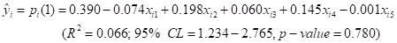 | |
| Overall estimated probability that the ith randomly selected mother has a gestation length lasted for less than 39.5 weeks | 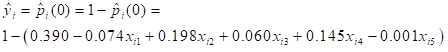 | |
 | Implies holding constant maternal age and gender (equating to zeros) of last birth, the expected probability is 14.5 percent higher on the average for a randomly selected mother with a parity of two or three children when compared with other mothers that their gestation length of their last birth is over 39.5 weeks. | |
 | Implies holding constant her parity and gender (equating to zeros) of her last birth, the expected probability is 7.4 percent lower on the average for a randomly selected mother with age 25 years or less when compared with other mothers that their gestation length of their last birth is over 39.5 weeks. | |
| Odds | Odds ratio | |
| The odds or probability that the ith randomly selected mother has a male birth with gestation period of more than 39.5 weeks | 0.636. | |
| The odds or probability that the last female birth of a randomly selected mother has a gestation period of more than 39.5weeks | 0.639 | |
| The odds ratio of male to female birth of a randomly selected mother having a gestation period of over 39.5weeks | 0.995 | |
| The odds or probability that the most recent (last) male birth by a randomly selected woman aged 30 years or more with more than three last births has a gestation length of over 39.5 weeks | 38.9 percent | |
| The odds or probability that the most recent (last) male birth by a randomly selected woman aged 30 years or more with more than three last births has a gestation length of equal to or less than 39.5 weeks | 61.1 percent | |
| The odds ratio that the most recent (last) male birth by a randomly selected woman aged 30 years or more with more than three last births has a gestation length of over 39.5 weeks or at most 39.6 weeks is 0.637and it implies that for every 1000 most recent male births with a gestation period of at most 39.5 weeks by women aged 30 years or more with more than three children we would expect about 637 of these most recent births to have a gestation period of over 39.5 weeks. | 0.637. | |
| The odds or probability that the most recent female birth by a randomly selected mother aged 30 years or more with more than three children has a gestation period of over 39.5 weeks | 0.390 | |
| The odds or probability that the most recent female birth by a randomly selected mother aged 30 years or more with more than three children has a gestation length at most 39.5 weeks | 0.61 | |
| Odds ratio that the most recent female birth by a randomly selected mother aged 30 years or more with more than three children has a gestation period of over 39.5 weeks or at most 39.5 weeks is 0.639 and it implies that for every 1000 most recent female births by a randomly selected mother aged 30 years or more with more than three children with a length of gestation of at most 39.5 weeks 639 of these female births are expected to have a length of gestation of over 39.5 weeks. | 0.639 | |
| The estimated odds ratio based on absolute probability interpretation is 0.997 implying that for every 1000 most recent female births with a length of gestation of over 39.5 weeks we would expect about 997 most recent male birth by mothers aged 30 years or over and with more than three children to also exceed a length of gestation of 39.5 weeks. | 0.997 | |
| The odds or probability that a randomly selected mother aged 25 years or less with a parity of at most one child has a male birth after 39.5 weeks of gestation is 37.5 percent. That is, the most recent birth by a randomly selected mother aged 25 years or less with a parity of at most one child, if male has a probability of 37.5 percent of being born after. | 37.5 Percent | |
| The odds or probability that a randomly selected mother aged 25 years or less with a parity of at most one child has a male birth at most 39.5 weeks of gestation is 62.5 percent. That is, the most recent birth by a randomly selected mother aged 25 years or less with a parity of at most one child, if male has a probability of 62.5 percent of being born before a gestation period of 39.5weeks. | 62.5 percent | |
| The estimated odds ratio based on absolute probability interpretation is the odds ratio of the probability that a randomly selected mother aged 25 years or less with a parity of at most one child has a male birth above 39.5 weeks of gestation to the probability that a randomly selected mother aged 25 years or less with a parity of at most one child has a male birth at most 39.5 weeks of gestation is 60 percent. This implies that for every 1000 most recent male births by mothers aged at most 25 years with not more than one child following a gestation period of at most 39.5 weeks there are 60 male births by these women with a gestation period of over 39.5 weeks. | 60 percent | |
| The odds that the most recent female birth by the randomly selected mother has a gestation period of over 39.5 weeks | 60.3 percent | |
| We can go on and on to estimate probabilities, odds and odds ratios of our desires using the same pattern | ||
Strength of Using Dummy Variable Regression Model in The Study
The following are the strength of dummy variable regression: (a). The dummy variable regression model effectively handled the categorical variables, namely maternal age, parity and gender by converting them into numerical variables, enabling analysis of their impact on gestation lengths. (b). The coefficients from dummy variable regression model provided insights into the differences between categories, allowing researchers to understand the relationships between variables. (c). In terms of flexibility, the model was used with gestation length data just as it can be suitably applied in other types of data. It also can accommodate multiple categorical variables which can make it versatile for analyzing complex relationships. (d). Because it is suitable for estimating probabilities and odds ratios, researchers can estimate probabilities and odds ratios for different categories which can provide valuable information for decision-making and prediction. (e). Dummy variable regression model helped us to understand the differences in gestation lengths between various categories of the predictor variables. (f). It quantified the relationships between categorical variables and gestation lengths, enabling us to identify significant associations. (g). Finally, by estimating probabilities and odds ratios of gestation lengths, one can inform decision-making and develop targeted interventions to improve birth outcomes.
Implications of The Study
The implications are: (a). A clear understanding of the determinants of gestation length can inform prenatal care and interventions to improve birth outcomes. (b). Estimating probabilities, odds and odds ratios can assist in identifying high-risk pregnancies which will facilitate targeted interventions and resource allocation. (c). Results obtained from this study can inform public health policy and programs that is aimed at improving maternal and child health outcomes in Ebonyi State. (d). This study is capable of providing methodological insights into the application of dummy variable regression model in analyzing data of length of gestation which will contribute to future research. (e). The limitations of this study can highlight some areas for future research which may include exploring other statistical models or incorporating additional variables.
Discussion
Recent research works highlight the importance of proper model fitting, validation, and diagnostics to ensure the accuracy and reliability of estimates. Papers published in the last few years discuss how to derive odds ratios from different model parameterizations, the application of dummy variable regression to analyze diagnostic screening tests, and methods to mitigate potential biases in odds ratio estimates from logistic regression. They also interpret odds ratios in a simplified manner. In line with this development, this study aimed at developing and using dummy variable regression to estimate probabilities, odds and odds ratios of gestation lengths of the most recent baby based on data from a cross-sectional study. The nature of the data is such that the outcome predictor variable (gestation lengths) is continuous while the predictor independent variables are categorical. This is a deviation from the usual approach of using logistic regression in determining the relationship between the binary outcome variable and independent categorical variables. Similarly, Lara et al [19] aimed at estimating measures of association between an exposure, health determinant or intervention, and a binary outcome by comparing the estimation and goodness-of-fit of logistic, log-binomial and robust Poisson regression models, in two cross-sectional studies involving frequent binary outcomes. They obtained Odds ratios (OR) through logistic regression, and prevalence ratios (PR) through log-binomial and robust Poisson regression models as well as confidence intervals (CI). In the two studies carried out, it was shown that the values of their OR and CLs are similar in comparison with what this found. They concluded that the odds ratio overestimated PR with wider 95% CI. The overestimation was greater as the outcome of the study became more prevalent, in line with previous studies. In one of the studies, the logistic regression was the model with the best fit, illustrating the need to consider multiple criteria when selecting the most appropriate statistical model for each study. Employing logistic regression models by default might lead to misinterpretations. They concluded in the study that Robust Poisson models are viable alternatives in cross-sectional studies with frequent binary outcomes, avoiding the non-convergence of log-binomial models. Hossain [14] used the logistic regression model in finding the factors associated with the likelihood of skilled workers in the garment sector of Bangladesh. This particular study adopted the pattern of interpreting the odds ratios as in this study. They result of odd ratios values showed that the male group is 3.0695 times more likely than the female group to be a skilled worker, which is significant at a 10% level; a group of rural workers is 10.3727 times more likely than the urban group in favour of skilled workers, which is significant at a 15% level; a group of workers have a training program degree is 38.5552 times more likely in favour of skilled workers, than a group of workers who have not, which is statistically significant at any significance level. According to Okeh and Onyeau [20], clinical practices allow for small sample sizes (n less than or equal 25) especially when there is need for a more exact result. In their comparison of two diagnostic tests, they concluded in their analysis that Modified Wilcoxon Signed Rank Test offered more reliable statistical inferences for small sample sizes of at most 25 and so is recommended as a permutation test as it provides a reliable result. Based on this fact, the use of sample size 41 in this cross-sectional study offered a reliable result of the gestation length been estimated. More so, statistically by Central Limit Theorem, a sample of an observational study is considered large if and only if the sample size is at least 30 (n greater than or equal to 30)
Summary and Conclusion
We have in this paper tried to develop an alternative method of estimating the probabilities, odds and odds ratios of the occurrence of continuous outcome variable using multiple dummy variable regression where the dependent (outcome variable) is continuous and independent variables are all categorical. Instead of the usual logistic regression approach, we applied a method that enables the interpretation of the resulting partial regression coefficients as probabilities. The proposed method does not require the often-restrictive assumptions of normality and homogeneity usually necessary when the outcome variables used in a regression model are assumed to be continuous. The method is illustrated with some sample data from a University Teaching Hospital in Ebonyi State where gestation length for last births is regressed against maternal age, parity and gender of last birth and the results were shown to compare favorably with results usually obtained using logistic regression.
Abbreviations
GDM: Gestational Diabetic Mellitus
ANOVA: Analysis of Variance
SS: Sum of Squares
DF: Degree of Freedom
MSE: Mean Square Error
Declarations
Acknowledgements
Thanks to the staff of the medical records of Alex Ekwueme Federal University Teaching Hospital Abakaliki Ebonyi State Nigeria for their assistance in making the data available for this research.
Funding
Thanks to TETFUND IBR Intervention fund for 2025 first Tranche release. The research was fully sponsored by this body.
Ethical approval
Not applicable since the privacy of the women were not involved.
Conflicts of Interest
Not applicable.
References
- Bajpai, P. (2013). Multiple regression analysis using ANCOVA in University model. International Journal of Applied Physics and Mathematics, 3(5):336.
Publisher | Google Scholor - Shpresa, S. Y. L. A. (2013). Application of Multiple Linear Regression Analysis of Employment through ALMP. International Journal of Academic Research in Business and Social Sciences, 3(12):2222-6990.
Publisher | Google Scholor - Nathans, L. L., Oswald, F. L., Nimon, K. (2012). Interpreting multiple linear regression: a guidebook of variable importance. Practical Assessment, Research & Evaluation, 17(9):n9.
Publisher | Google Scholor - Kelley, K., Maxwell, S. E. (2003). Sample size for multiple regression: obtaining regression coefficients that are accurate, not simply significant. Psychological Methods, 8(3):305.
Publisher | Google Scholor - Ludlow, L., Klein, K. (2014). Suppressor variables: The difference between is versus acting as. Journal of Statistics Education, 22(2).
Publisher | Google Scholor - Oyeka ICA, Okeh UM. (2013). Estimating Odds Ratios in Logistic Regression of Dichotomous Data. 2:608.
Publisher | Google Scholor - Delinda, M., Sari, D. P. (2023). University Election Analysis Logistic Regression Approach with Dummy and Ordinal Variables. Mathematical Journal of Modelling and Forecasting, 1(2):1-9.
Publisher | Google Scholor - Hua, Y., Stead, T. S., George, A., Ganti, L. (2025). Clinical risk prediction with logistic regression: Best practices, validation techniques, and applications in medical research. Academic Medicine & Surgery.
Publisher | Google Scholor - Muller, C. J., MacLehose, R. F. (2014). Estimating predicted probabilities from logistic regression: different methods correspond to different target populations. International Journal of Epidemiology, 43(3):962-970.
Publisher | Google Scholor - Moawed, S. A., El-Aziz, A. H. A. (2022). The estimation and interpretation of ordered logit models for assessing the factors connected with the productivity of Holstein–Friesian dairy cows in Egypt. Tropical Animal Health and Production, 54(6):345.
Publisher | Google Scholor - Sroka, C. J., Nagaraja, H. N. (2018). Odds ratios from logistic, geometric, Poisson, and negative binomial regression models. BMC Medical Research Methodology, 18(1):112.
Publisher | Google Scholor - Zhou, X., He, J., Wang, A., Hua, X., Li, T., et al. (2024). Multivariate logistic regression analysis of risk factors for birth defects: a study from population-based surveillance data. BMC Public Health, 24(1):1037.
Publisher | Google Scholor - K.A. Adeleke and A.A. Adepoju. (2010). Ordinal Logistic Regression Model: An Application to Pregnancy Outcomes. Journal of Mathematics and Statistics 6(3):279-285.
Publisher | Google Scholor - Hossain, M. S. (2023). Estimation of a logistic regression model to determine the effects of the factors associated with the likelihood of skilled workers in the garment sector of Bangladesh. European Journal of Business and Innovation Research, 11(7):1–34.
Publisher | Google Scholor - Usman, U., Waziri, M., Manu, F., Zakari, Y., & Dikko, H. G. (2021). Assessing the performance of some re-sampling methods using logistic regression. FUDMA Journal of Sciences, 5(1):445–456.
Publisher | Google Scholor - Boyle, R. P. (1970). Path analysis and ordinal data. American Journal of Sociology, 75(4):461–480.
Publisher | Google Scholor - Neter, J., Wasserman, W., & Christopher, N. (1974). Applied linear statistical models. New York, NY: McGraw-Hill.
Publisher | Google Scholor - Oyeka, I. C. A. (2013). Ties adjusted two-way analysis of variance tests with unequal observations per cell. Science Journal of Mathematics & Statistics, 2013(2013):1–6.
Publisher | Google Scholor - Pinheiro-Guedes, L., Martinho, C., & Martins, M. R. O. (2024). Logistic regression: Limitations in the estimation of measures of association with binary health outcomes. Acta Médica Portuguesa, 37(10):697–705.
Publisher | Google Scholor - Hossain, M. S. (2023). Estimation of a logistic regression model to determine the effects of the factors associated with the likelihood of skilled workers in the garment sector of Bangladesh. European Journal of Business and Innovation Research, 11(1):1–34.
Publisher | Google Scholor - Okeh, U. M., & Onyeagu, S. I. (2018). A modified Wilcoxon signed rank test for comparing ROC curves in a matched pair design. International Journal of Physical Sciences Research, 6(1):15–29.
Publisher | Google Scholor